ML learning notes (cmu10601) Lec1-2

prerequisite:

refer to https://www.cs.cmu.edu/~mgormley/courses/ml-primer/index.html

Lecture 1

1. Formulate a well-posed learning problem for a real-world task by identifying the task, performance measure, and training experience.

Define the problem as a tuple \langle \mathbf{T}, \mathbf{P}, \mathbf{E} \rangle.

Task (T): The function the system must learn (e.g., classifying images, predicting house prices).

Performance Measure (P): The metric to evaluate success (e.g., accuracy, precision, F1 score, root mean squared error (RMSE)).

Experience (E): The data the model learns from (e.g., a labeled dataset of images and their categories).

2. Describe common learning paradigms in terms of the type of data available, when it’s available, the form of prediction, and the structure of the output prediction.

Supervised Learning: Labeled data (x, y) available upfront. Predictions map input features (x) to discrete classes (Classification) or continuous values (Regression).

Unsupervised Learning: Unlabeled data (x) available upfront. Predictions reveal underlying structure (e.g., grouping data points via Clustering or dimensionality reduction).

Reinforcement Learning: No upfront dataset; agent learns through interaction with an environment (E) by receiving delayed rewards, aiming to maximize cumulative reward. Predictions are sequences of Actions or an optimal Policy.

3. Explain the difference between memorization and generalization

Memorization (Overfitting): A model performs exceptionally well on the Training Data (low training error) but fails on unseen data because it has learned the noise or idiosyncrasies specific to the training examples. It is unable to extract the true underlying pattern.

Generalization: A model has learned the essential, underlying patterns (the target concept) and is able to predict accurately on Unseen Data (low test/true error). Good generalization means the model is robust and useful in the real world.

Lecture 2

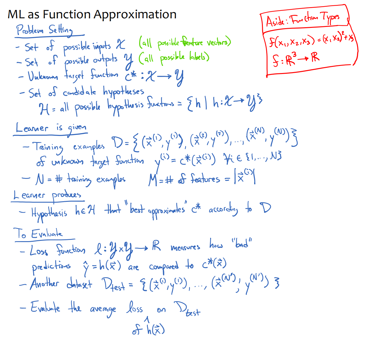
1. How do you mathematically formalize a Supervised Learning problem?

We define it as function approximation. Given a training set D, we search through a hypothesis space \mathcal{H} to find a function h(x) that best approximates the unknown target function c^*(x) by minimizing a specific loss function.

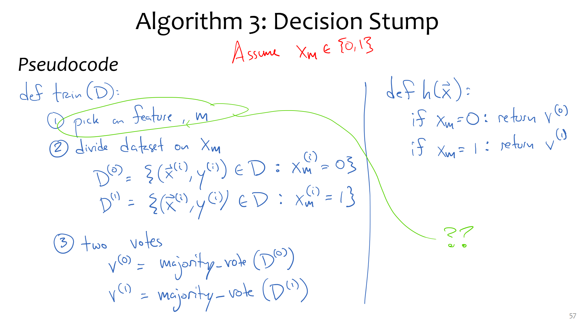
2. Describe the logic behind a simple rule-based classifier, like a Decision Stump.

A Decision Stump is a one-level decision tree that splits data based on a single feature. It iterates through all features to find the one that minimizes training error, predicting the majority class for each side of the split.

import numpy as np
from scipy import stats

class DecisionStump:
    def __init__(self):
        self.best_feature_index = None
        self.split_rules = {}  # Stores the prediction for each feature value
        
    def fit(self, X, y):
        """
        X: 2D array of features (rows are examples, cols are attributes)
        y: 1D array of labels
        """
        n_samples, n_features = X.shape
        best_accuracy = -1
        
        # 1. Iterate over every possible feature to split on
        for feature_index in range(n_features):
            current_rules = {}
            predicted_y = np.zeros(n_samples)
            
            # Get all unique values for this feature (e.g., 'Yes', 'No')
            unique_values = np.unique(X[:, feature_index])
            
            # 2. For each value, find the majority label (The "Vote" step)
            for val in unique_values:
                # Find indices where the feature equals this specific value
                indices = np.where(X[:, feature_index] == val)[0]
                
                # Find the most common label in this subset
                # (mode returns the most common value)
                majority_label = stats.mode(y[indices], keepdims=True)[0][0]
                
                # Store the rule
                current_rules[val] = majority_label
                
                # Save predictions for accuracy calculation
                predicted_y[indices] = majority_label
            
            # 3. Calculate accuracy for splitting on this feature
            accuracy = np.mean(predicted_y == y)
            
            # 4. Keep this feature if it's the best so far
            if accuracy > best_accuracy:
                best_accuracy = accuracy
                self.best_feature_index = feature_index
                self.split_rules = current_rules
                
        print(f"Training Complete. Best Feature Index: {self.best_feature_index}")
        print(f"Rules: {self.split_rules}")

    def predict(self, X):
        predictions = []
        for i in range(len(X)):
            feature_val = X[i, self.best_feature_index]
            # Retrieve the majority vote for this value
            pred = self.split_rules.get(feature_val)
            predictions.append(pred)
        return np.array(predictions)

# --- Example Usage based on Lecture Data ---
# Features: [Allergic, Hives, Sneezing, Red Eye, Has Cat] (Y=1, N=0)
X_train = np.array([
    [1, 0, 0, 0, 0], # Patient 1
    [0, 1, 0, 0, 0], # Patient 2
    [1, 1, 0, 0, 0], # Patient 3
    [1, 0, 1, 1, 1], # Patient 4
    [0, 1, 1, 0, 0]  # Patient 5
])

# Labels: Sick (+) = 1, Healthy (-) = 0
y_train = np.array([0, 0, 1, 0, 1]) 

# Train the model
stump = DecisionStump()
stump.fit(X_train, y_train)

# Output should show which feature (column) best separates Sick vs Healthy

3. Why is Inductive Bias necessary for a model to generalize?

Without inductive bias (assumptions about the data structure), a model acts like a Memorizer—it can only recall seen examples but cannot predict unseen ones. Bias constrains the hypothesis space (e.g., assuming the data is linearly separable) to enable generalization to new data.

4. Explain Overfitting using the concept of a 'Memorizer' algorithm.

A Memorizer achieves zero training error by storing every example perfectly. However, it fails completely on test data (high test error) because it learned the specific examples rather than the underlying pattern. This gap between low training error and high test error is the definition of overfitting.

5. How do we mathematically quantify how 'bad' a prediction is for different types of problems? (Loss Functions)

We use a Loss Function l(y, \hat{y}).

For Regression (real-valued outputs), we typically use Squared Loss: l(y, \hat{y}) = (y - \hat{y})^2

For Classification (discrete outputs), we use Binary or 0-1 Loss: l(y, \hat{y}) = \mathbb{I}(y \neq \hat{y}) (returns 1 if wrong, 0 if correct)

6. Why do we evaluate models on a Test Set instead of calculating the True Error directly? (The "Surrogate" Error)

We care most about the True Error (error_{true}(h)), which is the error over all possible inputs. However, because the target function c^*(x) is unknown for the entire population, the True Error is unknown in practice. Therefore, we use the error on a separate Test Dataset (error(h, D_{test})) as a surrogate (proxy) to estimate the true performance.

7. What is a 'Hypothesis Space' in the context of supervised learning?

The Hypothesis Space (\mathcal{H}) is the set of all candidate functions that the learning algorithm can possibly choose from.

Example: In the sine wave approximation task, \mathcal{H} was the set of all piecewise linear functions.

Example: For the diagnosis task, \mathcal{H} was the set of all possible decision trees.

Note：These notes are personal study notes based on publicly available machine learning lectures and textbooks. They are not solutions to any course assignments or examinations.